The U.S. House candidates who moved the needle in 2024

Announcing our new measure of candidate quality, the Wins Above Replacement Probability (WARP)

Editor’s note: Building on this newsletter’s increasing rate of collaboration with other smart, independent political analysts, today’s post is the result of a lot of behind-the-scenes work by me and Mark Rieke, a data scientist and blogger at The Data Diary. Mark has been working for some time now on a new measure of candidate quality in U.S. House elections, which I was happy to provide data for and feedback on, and which we now detail in this piece.

Both Mark and I wrote the piece, so I use collective nouns, but please give Mark all the credit for the modeling work — I formulated some parameters, but he wrote every line of code. Tomorrow, I’ll publish another analysis of these numbers for premium subscribers. The big question there: Do voters still reward ideological moderates?

Elliott

---

A short introduction to Wins Above Replacement

Today, Strength In Numbers is releasing our 2024 House estimates for two measures of candidate quality: Wins Above Replacement (WAR) and a new metric we’re introducing, Wins Above Replacement in terms of Probability (WARP).

WAR is a measure of how much better or worse a candidate for office performs, in terms of vote margin, compared to a hypothetical “replacement-level” candidate from the same party, for the same seat. WARP, on the other hand, is something entirely new we’ve cooked up that we think gets closer to what people actually care about: winning. Instead of measuring vote margin, WARP measures how much a candidate changes their party’s probability of winning a seat. If a candidate does much better than a hypothetical alternative, in a competitive seat, they get a high WARP.

WARP helps us separate margins that matter from margins that don’t. In safe districts, replacement-level candidates are unlikely to increase or decrease their party’s chances of winning the seat. So WAR can be incredibly high or drastically low while WARP remains at zero. In close races, however, a relatively small overperformance can drastically increase a party’s chance of winning the seat. WARP captures that nuance.

In addition to the inclusion of our new WARP metric, we think our model of WAR adds to the existing landscape in a few ways.

• More complete counterfactuals: Other popular models of politician WAR ignore the effects of challenger experience and do not disentangle fundraising from incumbent performance. But these variables can be crucial in measuring skill. Compared to other approaches, our model adds data on experience and treats both it and candidate fundraising as features when assessing hypothetical alternatives. This means candidates get more credit when they’re good fundraisers, relative to the replacement-level alternative, and less when they perform as expected against low-skill competitors.

• Separable candidate skill: Other models of WAR predict election results just using so-called “fundamentals” of the race (ie, no polls), and then call the errors of that model the WAR for each candidate. But we think that skill for the Democrat and Republican candidates in each race are different, so we measure each candidate’s underlying “skill” directly in the WAR/WARP model.¹ This lets us separately estimate the WAR/WARP values for both the Democratic and Republican candidates in each election, rather than assuming that one candidate’s skill implies the other candidate’s incompetence.

• Predictive WAR/WARP: The model only makes use of variables that are known prior to election day — it uses lagged presidential vote, demographics, incumbency, candidate experience, fundraising, and modeled candidate skill to estimate the outcome in each race and compute WAR/WARP. By only conditioning on variables known a priori, we can make reasonable statements about candidate quality prior to elections, rather than using WAR/WARP as a purely retrospective metric.²

• Quantifying Uncertainty: We estimate WAR using a probabilistic Bayesian model. Unlike other methods, which can only return point estimates for each candidate’s WAR, this approach allows us to quantify the uncertainty around each estimate and report WAR in terms of a median estimate and uncertainty interval.

In addition to everything above, the model and all pre/post-processing wrangling code is fully open source and available on GitHub! We think transparency encourages collaboration and fosters knowledge sharing, and we encourage enterprising readers to explore the source code in full detail. We are open to feedback.

WAR/P for all U.S. House Representatives

Here are the results!

(For now, we limit the table above to current House representatives, but plan to add a searchable database of all candidates for federal office soon.)

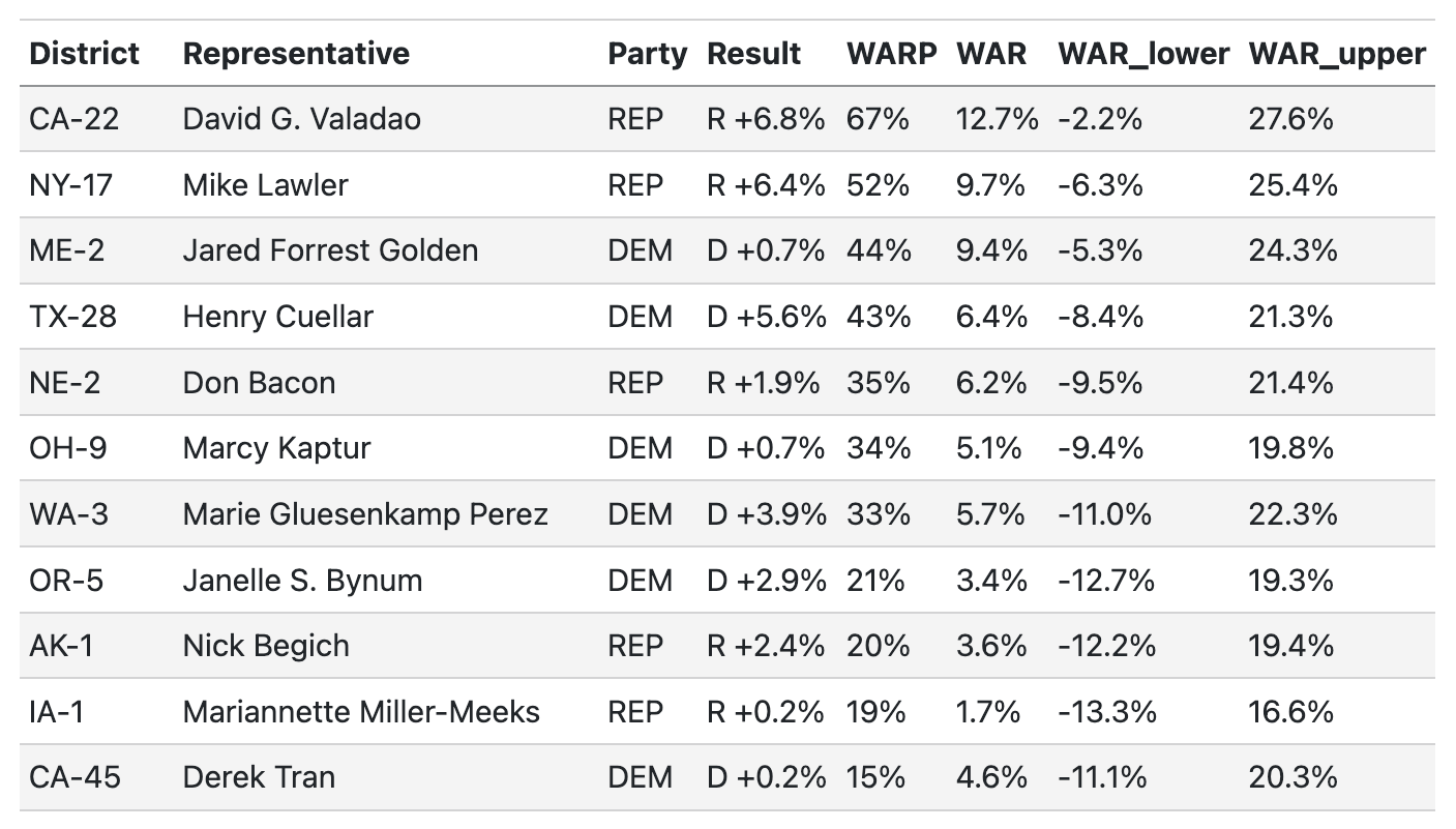
Per our model, David Valadao, the Republican representative from CA-22, was the most valuable candidate in 2024 in terms of WARP — Valadao was 67 percentage-points more likely to be elected than a hypothetical alternative Republican. By the same measure, ME-2’s Jared Golden was the most valuable Democratic representative with a WARP of 44%.

In terms of vote margins, candidates with high WAR (both positive and negative) mostly exist in safely held seats and have little effect on WARP. For example, we find that a typical republican would be expected to outperform Lauren Boebert in CO-4 by 8.6 percentage points, on average. Because the district is so red, however, both Boebert and a replacement would be nearly guaranteed to win.

This raises the question of whether you should look at WAR or WARP. In some practical situations, you’d want to use WAR; if Boebert switched districts, for example, you could use her WAR to predict under/overperformance in the new seat until you had information about the district’s voting behavior. Then, you could rep-predict her WARP with the new data.

Otherwise, you pretty much always want to use WARP. In general, as discussed above, WARP is a closer measure of winningness because it takes both seat characteristics and certainty into account.

Somewhat counterintuitively, it’s possible for a representative to have a negative WAR, on average, but still have a positive WARP. This is because sometimes the slightly lagging known candidate still has a better shot at winning than a completely unknown one. Take OR-6's Andrea Salinas, for example. A hypothetical alternative Democrat would be expected to, on average, increase the margin of victory in the district by 1.5 percentage points. Despite this, Salinas' WARP is positive — she is 8 percentage points more likely to win in the district than an alternative.

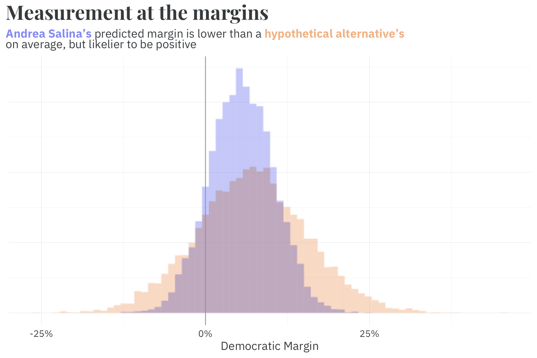
This is because the model has more precise information about Salinas than a hypothetical candidate. We have no idea who a replacement would be, and they could be quite a bit worse than Salinas. So, although the average predicted vote outcome with Salinas on the ballot is slightly less than the average prediction with an alternative, the more precise information gives us more certainty that Salinas' candidacy will result in a democrat winning the seat.

Ultimately, if you’re looking for a single number to evaluate a candidate’s value for their party in the seat they’re competing in, you should look at WARP, rather than WAR.

No coattails for Republicans in 2024

One of the narratives in the aftermath of the 2024 elections was that Republican house candidates underperformed Trump in their districts. Despite this underperformance relative to the top of the ticket, our results don’t suggest that Republicans writ large suffered due to issues of candidate quality. Across all races, representatives from both parties had very similar WARP scores:

• Democrats: 3.6%

• Republicans: 2.7%%

And in close races (decided by less than 10 percentage points), the average WARP was still incredibly similar:

• Democrats: 10.5%

• Republicans: 13.1%

By and large, Republicans didn’t concede large swathes of otherwise winnable seats to Democrats due to candidate quality issues. In fact, of the seats in which the result would have, on average, flipped to the other party if a replacement-level candidate had run, roughly half would have flipped to Democrats and half to Republicans:

We think this difference between the presidential and congressional results more likely points to Trump overperforming expectations, rather than downballot Republicans underperforming expectations. This view is consistent with pre-election forecasts from the likes of 538, where our (Elliott’s) median House forecast was incredibly close to the actual result, whereas the median national popular vote forecast underestimated Trump by about 3 percentage points on margin.

Our model tells a similar story. Conditional on only variables known before election day, both parties performed about as well as expected in the 2024 House elections. We don’t see evidence of a wave-level underperformance, just a close, competitive race for the house, with a few standout candidates improving their party’s chances around the edges.

---

Methodology

Our model is inspired by and an extension of the work of Lauderdale and Linzer (2015). We use hierarchical Bayesian regularization to include many predictors in the model without overfitting, time-varying parameters to account for changes in the electorate’s preferences from election to election, and introduce pairwise candidate comparisons to adjust for differences in candidate quality. The model is written in Stan, a probabilistic programming language for Bayesian inference.

1. Dealing with data

The model estimates the two-party vote share for all regularly scheduled congressional races from 2000-2024 where both a Democrat and a Republican appear on the ballot.³ In jungle primaries where a candidate does not win a majority of the vote in the first round, we model the results of the general election (provided that each party has a candidate representing them in the general). While not used for fitting the model, we do estimate WAR/WARP for candidates in uncontested races for completeness’s sake.

2. Model Mechanics

Our model estimates three outcomes simultaneously:⁴

• The outcome of the race in terms of the Democrats’ share of the two-party vote;

• The share of individual FEC contributions in the seat (provided FEC filings are available); and

• Whether or not non-incumbent candidates have held an elected office before.

The voteshare model is the most involved in terms of model complexity and is ultimately the main outcome of interest. But the FEC and experience models⁵ are necessary components that allow us to generate realistic hypothetical candidates when constructing counterfactual observations to estimate WAR/WARP. These additional models are one of the things that make our approach more accurate than others.

2.1 The vote share model

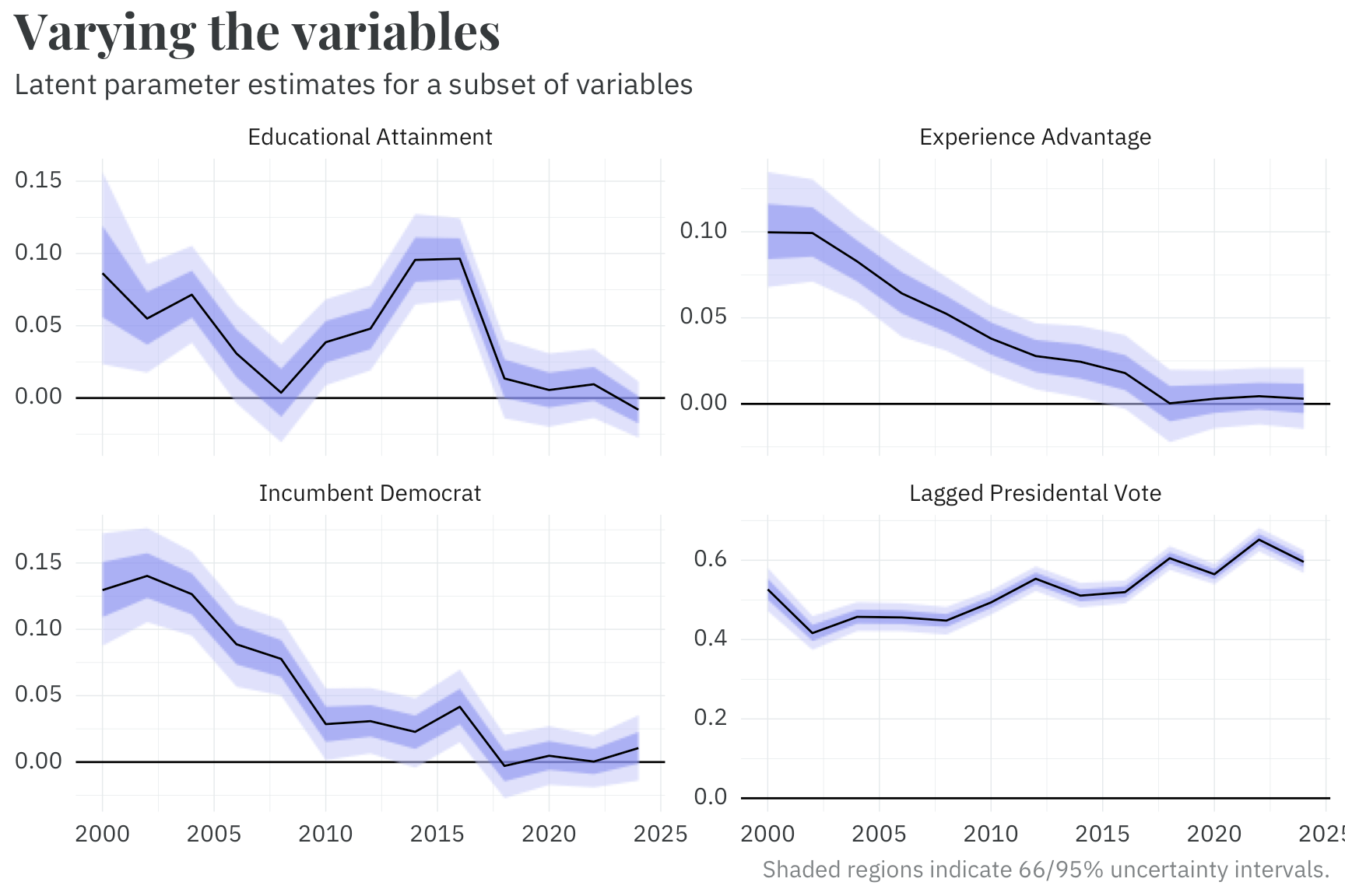
We use a wide range of variables that reflect the qualities of each candidate, the district, and the national environment to estimate the results of each congressional election. For a majority of these variables, we use a random walk that allows the parameter values of each predictor to drift from cycle to cycle.

As an interesting artifact, we find that, with the exception of lagged presidential vote, the model’s measurement of partisanship, most parameter values have drifted towards zero in recent years. If you know how a district voted in the previous election, that tells you most of what you need to know about which party it’ll vote into Congress!

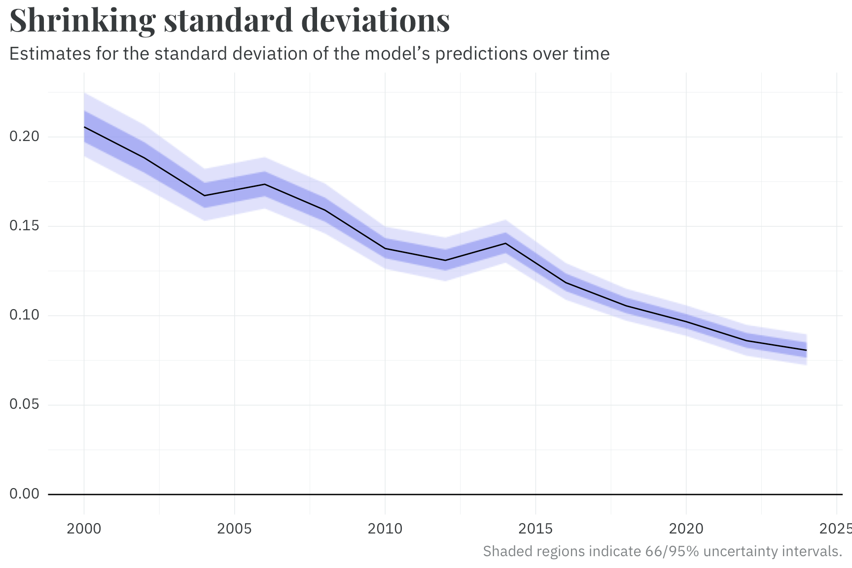
Similarly, the standard deviation of the estimated voteshare is allowed to change cycle-to-cycle — again, using a random walk. We find that this parameter, too, has been shrinking in recent years. In the most recent elections, our model is far more certain in the predicted outcome than its predictions in the early 2000s.

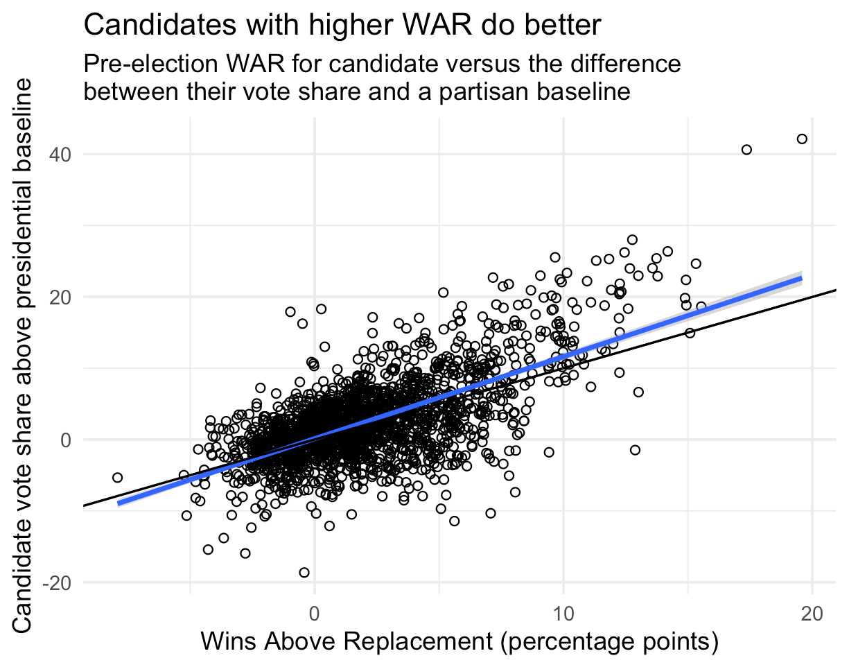
Finally, the voteshare model adjusts the estimates for predicted voteshare based on the difference in candidate skill parameters. This lets us encode the idea that, for example, in an otherwise coin-toss race, a highly skilled candidate will handily win when facing a low-skilled candidate. But in that same election, a match up between two low-skilled candidates or two high-skilled candidates will remain a tossup.

Unlike many of the other parameters of this model, the candidate skill parameters are static over time. Allowing candidate skill to vary over time is a theoretically attractive proposition — you can imagine a candidate getting better at campaigning after they adjust to serving in Congress or a scandal negatively affecting their ability to pull in votes. For a few practical reasons that I’ve relegated to the footnotes,⁶ however, we instead elect to use static parameters.

2.2 Fundraising model

Because there is missingness in our training data (some candidates do not disclose their FEC contributions, and data quality degrades for election earlier in the training set), we use a hurdle model⁷ to estimate both the probability that fundraising information is available for a race and the share of individual FEC contributions going to the Democratic candidate. Candidate experience and incumbency are used to estimate the share of FEC contributions — inexperienced candidates and non-incumbents tend to be outraised by experienced candidates or incumbents. The probability that FEC filing information is available is simply modeled as a random walk over year.

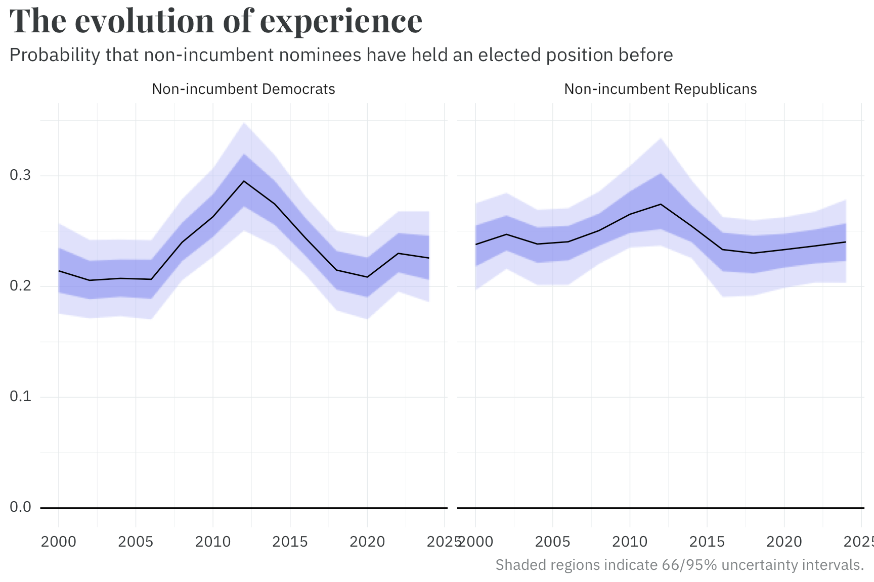
2.3 The experience model

By comparison, our model of candidate experience (whether they have previously won any elected office — eg, for mayor, state house, etc.) is relatively straightforward. We use this to predict the skill of a hypothetical replacement candidate, conditional on their party. We also allow this probability to vary over time via — you guessed it — another random walk. Interestingly, both parties peaked in terms of nominating candidates with prior experience around the same time in the early 2010s.

3. Constructing a good counterfactual

To estimate each candidate’s WAR/WARP, we need to generate:

• The candidate’s predicted vote share given everything we know about them, their competitor, and the district their running in; and

• The predicted vote share of a hypothetical alternative candidate.

For the actual candidate, this is fairly straightforward; we can simply use the results of the model to make a prediction of their expected vote share. The hypothetical alternative, however, is a bit more involved. We need to take care in ensuring that our counterfactual candidate correctly encodes the uncertainty we have about the qualities that they bring to the table: their experience, ability to fundraise, and individual skill. In practice, this means we need to run the entire model fitting process described above, but in reverse.

For every candidate, we perform the following steps:

First, we simulate whether or not our hypothetical candidate has previously held an elected position. In the vote share model, our experience variables are comparisons between the candidates — we predict the outcome based on whether the candidate had an experience advantage, disadvantage, or was evenly matched with their opponent. We do the same for our hypothetical candidate, comparing their experience against their opponent’s and recording which (if either) is the more experienced candidate.

Next, the model uses the simulated experience of each candidate to simulate the counterfactual share of FEC contributions. Much like experience, this variable depends on both the hypothetical candidate and their opponent. The model first simulates whether or not the hypothetical candidate has individual FEC contributions.

• If they do…

  • And their opponent has individual FEC contributions, the model simulates a new counterfactual share of FEC contributions for the race.

  • But their opponent doesn’t have individual FEC contributions, we set the hypothetical candidate’s counterfactual share of FEC contributions to ~100%.

• If they don’t…

  • But their opponent has individual FEC contributions, we set their opponent’s counterfactual share of FEC contributions to ~100%.

  • And their opponent doesn’t have individual FEC contributions, we ignore FEC information altogether for this counterfactual race.

The final step before the model can predict the vote share with this hypothetical candidate is to simulate their skill. Having learned what the distribution of skill values for other candidates looks like during the fitting process, the model simulates a new skill value for our hypothetical candidate from this distribution.

With all the necessary information to build out the counterfactual candidate’s profile now simulated, the model uses this information, along with district and national predictors, to simulate a potential outcome for the race with this replacement candidate on the ballot. WAR is then simply the difference between the two simulated values — the vote share with the actual candidate on the ballot minus the vote share with the hypothetical alternative on the ballot.

The model then repeats this entire process — simulating the actual candidate’s vote share, building out a counterfactual candidate profile to simulate the alternative’s vote share, and taking the difference — thousands of times to reflect our uncertainty in the process. WARP is the proportion of simulations in which the actual candidate wins the election minus the proportion of simulations where the alternative wins.

In conclusion

If you’ve gotten this far and are looking for more, we encourage you to go poking around in the model’s results. Although we don’t display it here, we’ve calculated WAR and WARP for every winner of every U.S. House election since 2000. If you have further methodological questions, please reach out to contact@gelliottmorris.com.

---

Footnotes

1. With a small caveat — for both computational efficiency and identifiability, we only model the individual skill of candidates who have ever served in Congress or have run for Congress multiple times. All others are considered a “generic challenger” by the model.

2. Our model’s predictive WAR/WARP performs incredibly well on out-of-sample data.

3. With some reasonable exceptions for re-caucusing independents to one party. Specifically, Bernie Sanders is modeled as a Democrat, despite running as an independent candidate.

4. Or, to use the technical Bayesian lingo,™ we model these outcomes jointly.

5. I should note that, although I refer to the voteshare, FEC, and experience components of the model separately, they really are all part of one big model! In contrast with fitting models separately and using the outcome of one model as the input to another, the “one big model” approach straightforwardly propagates uncertainty through the submodels.

6. There is simply not enough data to reliably estimate these time-varying parameters. A representative who has served in congress since 2000 — as far back as our dataset goes — only has 13 elections from which we can try to infer skill.

• We would end up having to write a (very) computationally inefficient model. Some candidates appear in all election cycles, but most do not. Stan, our programming language of choice, doesn’t support ragged arrays — we cannot include variables that have differing numbers of observations (elections) per entry (candidate). We would instead have to include parameters for all election cycles per candidate, even if that candidate only appears in one election.

• Yes, yes, yes, I’m aware that there are technically some ways around this without introducing a bunch of extra parameters. The problem is that my prior note about having a maximum of 13 observations per candidate still stands. But more importantly, I wasn’t going to suffer an additional level of array indexing hell without some serious upside in terms of fit quality.

7. Submodels within submodels within models — truly I have become the Bene Gesserit here. (Okay, I also realize that the linked quote is said by the Baron and not one of the Bene Gesserit. But at this point, you’re reading a parenthetical within a footnote within an article. Just let me have this one.)